Optimizing School Locations with the P-Median Algorithm in KNIME
A practical introduction to location-allocation analysis using the KNIME Geospatial Analytics Extension
Why Location Allocation Matters
Every day, organizations make decisions about the locations of facilities. Where should a new retail store open? Where should EV charging stations be installed? Where should new schools be built? Although these seem like very different questions, they all have one thing in common: they aim to find the optimal balance between demand and supply. Which retail location gives access to the largest customer base? Which charging stations serve the highest number of electric vehicles? Which school locations minimize the travel distance for students? This class of optimization problems is known as Location Allocation. In this article I’ll solve one of the best-known location allocation problems, the P-Median problem, using the KNIME Geospatial Analytics Extension.
The P-Median Problem
To demonstrate the P-Median algorithm, I’ll use a simple but realistic example. Imagine a municipality wants to build a number of new primary schools. The municipality already has a list of potential school locations and knows how many children live in each neighbourhood. The challenge is to select exactly p school locations so that, on average, children have to travel as little as possible. As possible, because there may be other constraints on the table, like the maximum number of schools or the minimum number of children a school serves.
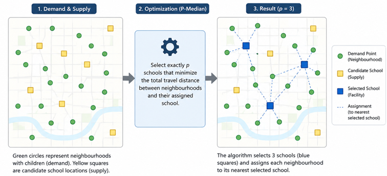
For this classic location allocation problem I’ll use the P-Median algorithm. The P-Median problem is one of the best-known models within the location allocation family. Given a number of demand locations and a set of candidate facility locations, the objective is to select exactly p facilities such that the total weighted travel cost between demand and the selected facilities (supply) is minimized (see figure *).
Demand and Supply
Every P-Median problem consists of two sets of locations. In this school location example, these can be defined as follows:
Demand
- Neighbourhoods
- Number of children
- Each neighbourhood represents a demand location with a demand value
Supply
- Candidate school locations
- Not every candidate location will be selected
To solve this location allocation problem, the P-Median node in KNIME requires only a limited number of input parameters (see the configuration dialog below).
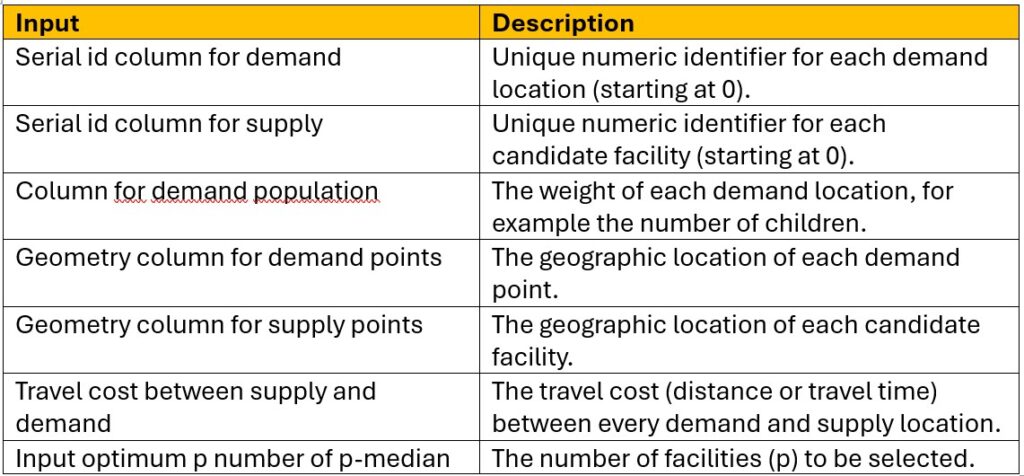
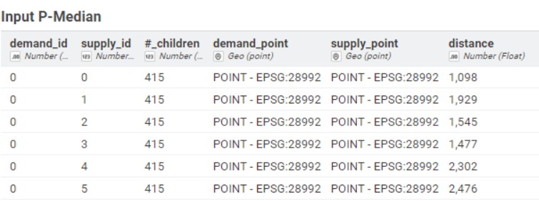
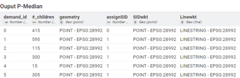
The P-Median node assigns every demand location to its nearest selected facility. The output therefore not only identifies which facilities have been selected, but also shows how every neighbourhood is allocated to one of these facilities. The output of the P-Median node contains everything needed to analyse and visualise the solution. For every neighbourhood, the selected school is identified together with the corresponding geometry.
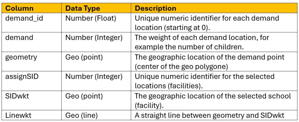
The output also contains a LineString (Linewkt) connecting every demand point with its assigned facility. Although this line does not represent the actual road route, it provides an intuitive visualization of the allocation.
What surprised me is how little configuration the P-Median node actually requires. The real challenge is not configuring the algorithm itself, but preparing the right input data: a demand set, a supply set and a realistic travel cost matrix. Once these are available, running the optimization becomes remarkably straightforward.
Implementing the P-Median analysis in KNIME
For this use case, I built a KNIME workflow, which is available for download from the KNIME Hub . Figure 3 shows the complete workflow.
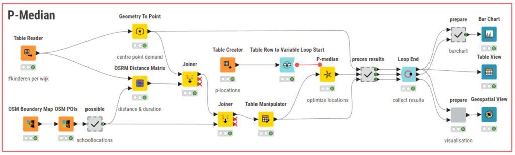
The workflow consists of four logical steps:
- Read the demand and supply datasets.
- Calculate the travel cost matrix using OSRM (Open Source Routing Machine)..
- Run the P-Median optimization.
- Analyze and visualize the results.
Why Travel Cost Matters
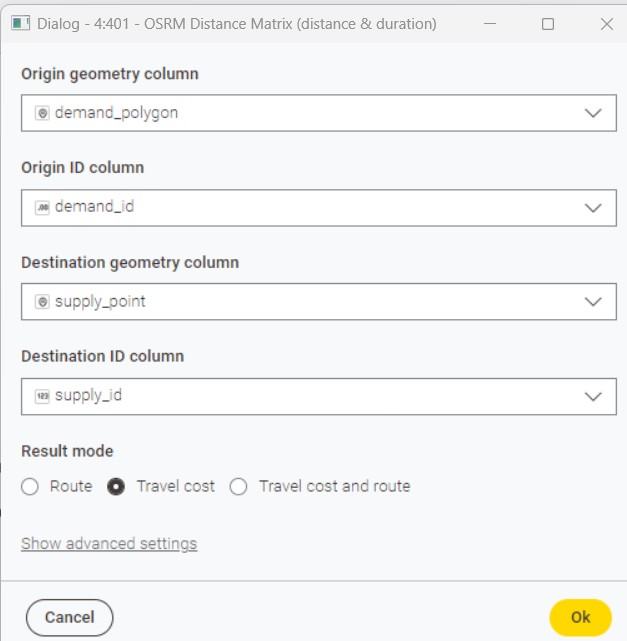
In this example, the optimization is based on the road network rather than on straight-line (Euclidean) distance. This results in a much more realistic representation of the travel distance between neighbourhoods and schools. The OSRM Distance Matrix KNIME node is also not complicated to configure. It gives you both distance and duration. And there is the option to retrieve the route (Geo line) between origin and destination. For this use case I used the distance as the feature to optimize.
More than a map
The output is not limited to a map. Because every neighbourhood is linked to a selected school, it becomes straightforward to calculate additional performance indicators, such as:
- the number of children assigned to each school;
- the average travel distance;
- the maximum travel distance;
- the expected capacity per school.
Comparing different scenarios
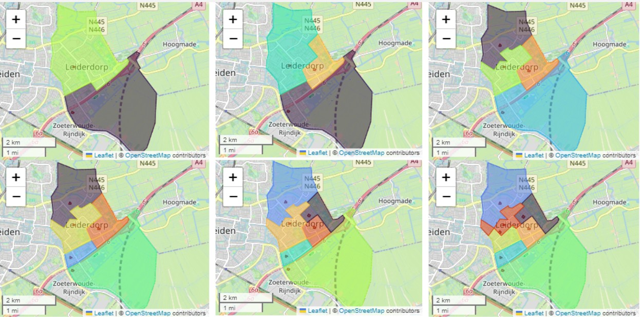
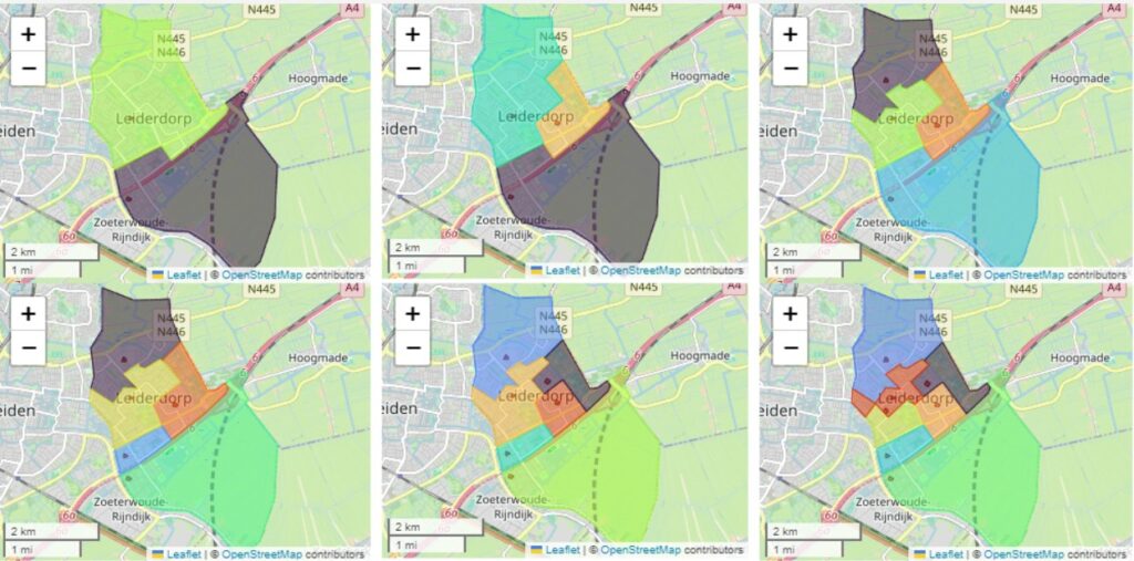
The P-Median algorithm assumes that the number of facilities (p) is known in advance. But how do you know whether three schools are enough? Or would four or five schools provide a significantly better solution? In practice, however, this is often exactly the question decision makers want to answer.
Instead of running the optimization manually for each value of p, I parameterized the number of facilities and used a Table Row to Variable Loop Start node to execute the workflow automatically for every scenario. This made it possible to calculate and compare multiple solutions in a single run.
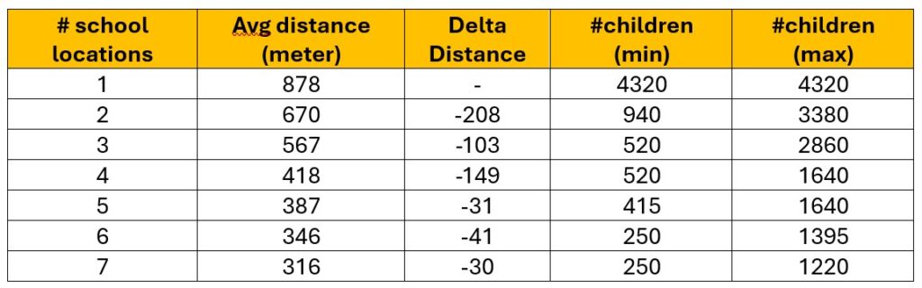
After about four schools, the reduction in average travel distance starts to level off (see Figure ), indicating diminishing returns. This suggests that scenarios with four or more schools deserve closer attention.
The results also raise an interesting follow-up question. Even with seven schools, one location still serves more than 1,200 children, while another serves only 250. If these numbers fall outside the municipality’s preferred capacity range, the current set of candidate locations may not be optimal. Rather than simply increasing the number of schools, planners could investigate whether alternative candidate locations would lead to a more balanced distribution of students while maintaining acceptable travel distances
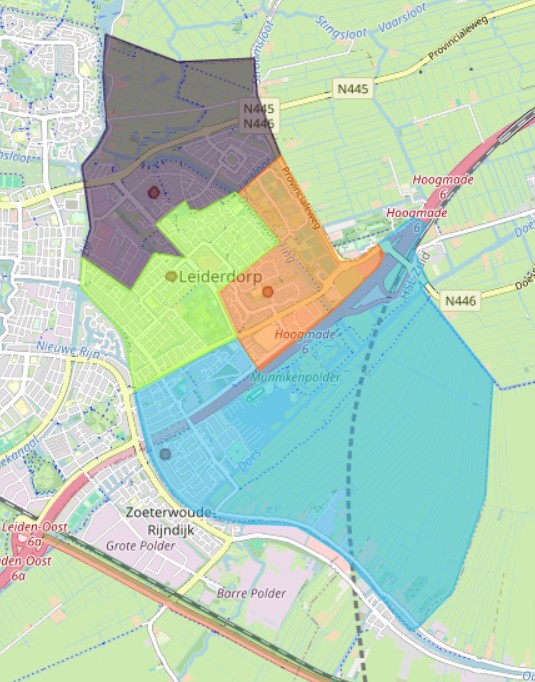
This illustrates an important point: optimization models answer the question you ask, but they also help reveal better questions.
Ultimately, KNIME doesn’t make the decision; it provides the evidence needed to make an informed one. Decision makers can weigh improved accessibility against the costs of opening and operating additional schools, or investigate whether alternative locations would provide a better overall solution. In other words, solving one optimization problem often reveals the next question worth exploring.
One of the most valuable outcomes of this analysis was not the “optimal” solution itself, but the realization that the predefined candidate locations may not be optimal. The analysis therefore becomes the starting point for a new round of exploration rather than the end of the decision-making process.
Why I like this approach
What I appreciate most about this KNIME workflow is that it combines geospatial analysis, optimization and data analytics in a single environment. From preparing the input data and calculating realistic travel distances to comparing multiple scenarios and visualizing the results, every step is captured in one transparent and reproducible workflow. This not only makes the analysis easier to understand, but also much easier to maintain, share and extend.
Although this example focuses on schools, exactly the same workflow can be applied to many other location allocation problems, including fire stations, healthcare facilities, parcel lockers, libraries, EV charging stations and retail stores. Only the input data changes; the workflow remains essentially the same.
More information
The P-Median node is only one of several Location Allocation algorithms available in the KNIME Geospatial Analytics Extension. Other optimization nodes include LSCP, MAEP and P-Center, each designed for different optimization objectives.
For more info about the KNIMÉ GeoSpatial nodes, take a look at:
https://hub.knime.com/knime/collections
https://www.knime.com/files/geospatial_analytics_cheatsheet.pdf